The psychological and genes’ eye view of ergodicity economics

This post was my plan for a presentation at the Foundation of Utility and Risk Conference. I drew on my previous posts laying out the foundations of ergodicity economics and examining what ergodicity economics states about risk preferences. This varied somewhat from delivery (I’m easily waylaid and skipped a couple of sections). Given it’s to a technical audience, there are a few moments that might lose the lay reader.

–

Introduction

This presentation started with a blog post. Around five years ago when I was ensconced in the corporate world, I wrote a couple of posts on an idea called ergodicity economics. A random physicist, Ole Peters, was riling people up on twitter about how economists were doing it wrong, how expected utility theory was fatally flawed, how you don’t need to introduce psychology to explain human decisions under risk, and how all the anomalies in behavioural economics could be reconciled with his new theory.

There were plenty of people countering the stronger statements, but I thought that by writing a post or two I could understand the idea better myself. So I ignored the hyperbole and tried to give a fair hearing to the underlying idea. Since I had some background in evolutionary biology, I also tried to view it from an evolutionary lens.

In the spirit of those original posts, I am going to avoid today’s presentation from becoming an exercise in attacking the most outlandish statements. There are a couple of published critiques of ergodicity economics, one by Jason Doctor et al (2020) in Nature Physics and one more recent by Matthew Ford and John Kay (2023) in Econ Journal Watch that do a good job of addressing the claims about economics and expected utility theory. Instead, I’m going to give a flat description of ergodicity economics, before laying out some psychological and evolutionary observations.

The bet

So let me start with the classic example used to illustrate what ergodicity economics is about. You may have seen this before.

Suppose you are offered a series of 100 bets on the flip of a coin. You win 50% of your wealth on heads. You lose 40% of your wealth on tails. Do you take the bet?

The expected value of the bet is 5% of your wealth each flip. Continue playing for many rounds and your expected wealth is very large.

However, what is the most probable outcome over many repeats of this bet?

This plot is the result of a simulation of 10,000 people, each starting with $100, experiencing the 100 flips. The black line is the average wealth of the population. The red lines are paths of the first 20 people in the simulation.

# Load the required packages

library(ggplot2)
library(scales) #use the percent scale later
library(dplyr) #use the filter function later

# Create a function for running of the bets.

bet <- function(p, n, t, start=100, gain, loss, ergodic=FALSE, absorbing=FALSE){

  #p is probability of a gain
  #n is how many people in the simulation
  #t is the number of coin flips simulated for each person
  #start is the number of dollars each person starts with
  #if ergodic=FALSE, gain and loss are the multipliers
  #if ergodic=TRUE, gain and loss are the dollar amounts
  #if absorbing=TRUE, zero wealth ends the series of flips for that person

  params <- as.data.frame(c(p, n, t, start, gain, loss, ergodic, absorbing))
  rownames(params) <- c("p", "n", "t", "start", "gain", "loss", "ergodic", "absorbing")
  colnames(params) <- "value"

  sim <- matrix(data = NA, nrow = t, ncol = n)

  if(ergodic==FALSE){
    for (j in 1:n) {
      x <- start
      for (i in 1:t) {
      outcome <- rbinom(n=1, size=1, prob=p)
      ifelse(outcome==0, x <- x*loss, x <- x*gain)
      sim[i,j] <- x
      }
    }
  }

 if(ergodic==TRUE){
    for (j in 1:n) {
      x <- start 
      for (i in 1:t) {
      outcome <- rbinom(n=1, size=1, prob=p)
      ifelse(outcome==0, x <- x-loss, x <- x+gain)
      sim[i,j] <- x
      if(absorbing==TRUE){
        if(x<0){
          sim[i:t,j] <- 0
            break
        }
        }
      }
    }
  }

  sim <- rbind(rep(start,n), sim) #placing the starting sum in the first row
  sim <- cbind(seq(0,t), sim) #number each period
  sim <- data.frame(sim)
  colnames(sim) <- c("period", paste0("p", 1:n))
  sim <- list(params=params, sim=sim)
  sim
}

# Simulate 10,000 people who accept a series of 1000 50:50 bets to win \$50 or lose \$40 from a starting wealth of \$100.

set.seed(20240705)
nonErgodic <- bet(p=0.5, n=10000, t=1000, gain=1.5, loss=0.6, ergodic=FALSE)

# Function to plot individual paths and average wealth over a set number of periods.
plotWealth <- function(sim, t = 100, people = NULL) {
  basePlot <- ggplot(sim$sim[1:(t+1),], aes(x = period)) +
    labs(y = "Wealth ($)")

  # Add lines for individual paths if specified
  if (!is.null(people)) {
    for (i in 1:people) {
      basePlot <- basePlot +
        geom_line(aes(y = !!sim$sim[c(1:(t+1)), i+1]), color = "red")
    }
  }

  # Add line for average wealth
  basePlot <- basePlot +
    geom_line(aes(y = rowMeans(sim$sim[1:(t+1), 2:(sim$params[2,]+1)])), color = "black", linewidth = 1)
  
  basePlot
}

# Generate the plot with individual paths and average wealth
nonErgodicPlot <- plotWealth(sim = nonErgodic, t = 100, people = 20)
nonErgodicPlot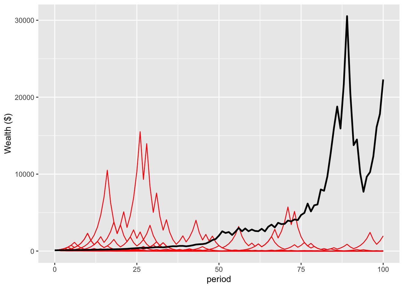

Figure 1: Plot of first 20 people against average wealth

The sudden drop in mean wealth toward the end of the sequence is an interesting feature that I will ignore for the moment. But look at the red lines. At the end of 100 periods, all are below the mean wealth, and only one of the 20 agents has enough wealth at the end that you can discern the line from the x-axis.

Let us now use a log scale to enable us to see the pattern more clearly.

# Plot both the average outcome and first twenty people on the same plot.

logNonErgodicPlot <- plotWealth(sim=nonErgodic, t=100, people=20)+
    scale_y_log10(breaks = c(0.0001, 0.1, 100, 100000), labels = c("0.0001", "0.1", "100", "100000"))
logNonErgodicPlot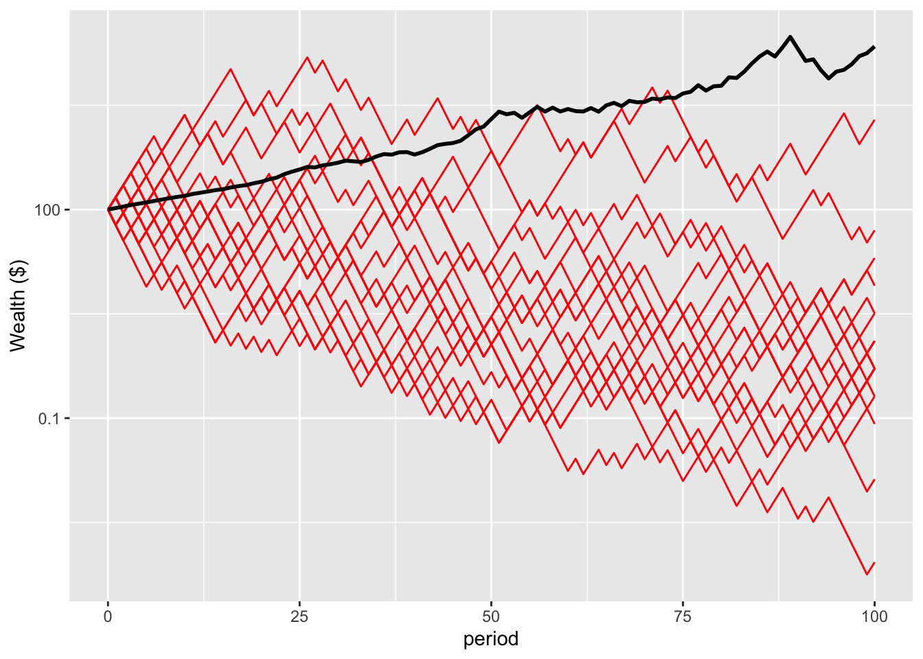

Figure 2: Plot of first 20 people against average wealth (log scale)

All 20 of these people are below the mean wealth. Only one is ahead of where they started.

# Create a function to generate summary statistics.
summaryStats <- function(sim, t = 100) {
  
  # Extract the wealth data for the specified time
  wealth_data <- as.matrix(sim$sim[(t + 1), 2:(sim$params[2, ] + 1)])
  
  # Calculate mean wealth
  mean_wealth <- mean(wealth_data)
  
  # Calculate median wealth
  median_wealth <- median(wealth_data)
  
  # Number and percentage who lost more than 99% of their wealth
  num_lost_99 <- sum(wealth_data < (sim$params[4, ] / 100))
  perc_lost_99 <- (num_lost_99 / sim$params[2, ]) * 100
  
  # Number and percentage who gained wealth
  num_gain <- sum(wealth_data > sim$params[4, ])
  perc_gain <- (num_gain / sim$params[2, ]) * 100
  
  # Number who increased their wealth more than 100-fold
  num_increased_100 <- sum(wealth_data > (sim$params[4, ] * 100))
  
  # Wealth and wealth share of the wealthiest person
  max_wealth <- max(wealth_data)
  perc_max_wealth_share <- max_wealth / sum(wealth_data) * 100
  
  # Combine all statistics into a data frame
  stats <- data.frame(
    mean_wealth = mean_wealth,
    median_wealth = median_wealth,
    num_lost_99 = num_lost_99,
    perc_lost_99 = perc_lost_99,
    num_gain = num_gain,
    perc_gain = perc_gain,
    num_increased_100 = num_increased_100,
    max_wealth = max_wealth,
    perc_max_wealth_share = perc_max_wealth_share
  )
  
  return(stats)
}


nonErgodicStats <- summaryStats(nonErgodic, 100)

These 20 people are representative of the broader population. Across the 10,000 agents in this simulation, 86 per cent lost money. The mean wealth was $22303, but the median wealth was $0.52.

What is the intuition behind this?

The black line reflects the expected gain of 5% per flip.

But for the red lines, over the long term, an individual will tend to get around half heads and half tails. As the number of flips goes to infinite, the proportion of heads or tails “almost surely” converges to 0.5. This means that each person will tend to get a 50% increase half the time (or 1.5 times the initial wealth), and a 40% decrease half the time (60% of the initial wealth). The time average growth in wealth for an individual is (1.5\times 0.6)^{0.5} \sim 0.95, or approximately a 5% decline in wealth each period. Every individual’s wealth will tend to decay at that rate. The black line is held up by a very lucky few.

A system where the time average converges to the ensemble average (our population mean) is known as an ergodic system. The sequence of gambles I have just shown you is non-ergodic as the time average and the ensemble average diverge. (I’ll ignore the finer debates about whether this problem even involves ergodicity to the side.)

This leads to the following claim: as we cannot individually experience the ensemble average, the ensemble average is not what humans consider in their decision making. Instead, people maximise the time average growth rate of wealth. For this bet, as the time average growth rate is negative, an ergodicity economics agent would reject the bet.

Contrast this with the expected utility approach, where the utility of each outcome is weighted by its probability and summed to give the expected utility. Expected utility theory would be consistent with both accepting and rejecting the bet depending on the particular utility function.

There is, however, an incidental alignment between ergodicity economics and expected utility theory. If a person has log utility - that is, they maximise the probability-weighted logarithm of the possible outcomes - they will maximise the time average growth rate.

Additive versus multiplicative

One important feature of the bet I have just shown is that the outcomes are multiplicative. A win on one flip leads to a larger stake flip on the next bet. The size of the bet scales up or down with wealth.

What if I offered you the following bet instead?

You have $100 and are offered a gamble involving a series of 100 coin flips. For each flip, heads will increase your wealth by $50. Tails will decrease it by $40. Do you take the bet?

You can see the tweak from the original bet, with dollar sums rather than percentages. For someone with $100 in wealth, the first flip is effectively identical, but future bets will be additive on that result and always involve the same shift of $50 up or $40 down.

This second series of flips is ergodic. The expected value of each flip is $5 (0.5\times \$50-0.5\times \$40=\$5). The time-average growth rate is also $5.

Let’s simulate as we did for multiplicative bets, with 10,000 people starting with $100 and flipping the coin 100 times. This plot shows the average wealth of the population, together with the paths of the first 20 of the 10,000 people (in red).

# Simulate 10,000 people who accept a series of 1000 50:50 bets to win \$50 or lose \$40 from a starting wealth of \$100.

set.seed(20240705)
ergodic <- bet(p=0.5, n=10000, t=100, gain=50, loss=40, ergodic=TRUE, absorbing=FALSE)

# Plot both the average outcome and first twenty people on the same plot.

ergodicPlot <- plotWealth(sim=ergodic, t=100, people=20)
ergodicPlot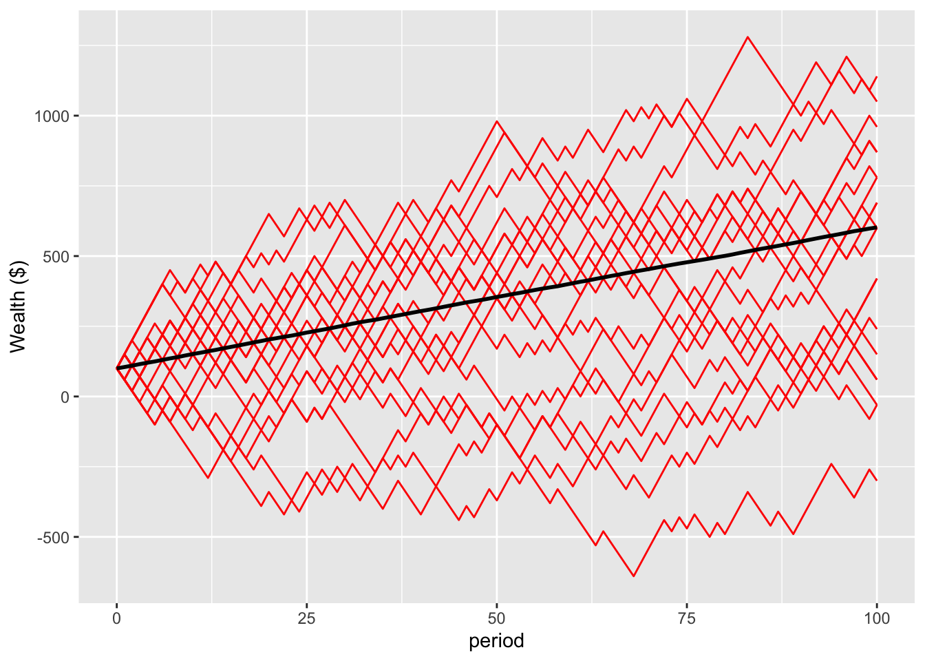

Figure 3: Average wealth of population and path of first 20 people

# Generate summary statistics for the population and wealthiest person after 100 and 1000 flips}

summaryErgodic100 <- summaryStats(sim=ergodic, t=100)

The individual growth paths cluster on either side of the population average. After 100 flips, the mean wealth is $602 and the median $600. 87% of the population has gained in wealth. This alignment between the mean and median wealth, and the relatively equal distribution of wealth, are characteristic of an ergodic system.

# Determine how many people (in the first people out of n) experienced zero wealth or less during the simulation.

numZero <- function(sim, t, subset=0){

  #subset
  data <- if(subset==0 | subset>sim$params[2,]){
    sim$sim[1:t,2:(sim$params[2,]+1)]
  } else {
    sim$sim[1:t,2:(subset+1)]
  }
  
  # number of people who experienced zero wealth or less
  numZero <- length(data) - sum(sapply(data, function(x) all(x>0)))
  numZero
  
}

numZeroTwenty100 <- numZero(sim=ergodic, t=100, subset=20)
numZeroTwenty1000 <- numZero(sim=ergodic, t=1000, subset=20)
numZero100 <- numZero(sim=ergodic, t=100)
numZero1000 <- numZero(sim=ergodic, t=1000)

Now for a wrinkle, which we can see in the plotted figure. Of those first 20 people plotted on the chart, 11(!) had their wealth go into the negative over those 100 periods. We see the same phenomenon across the broader population, with 5433 dropping below zero in those first 100 periods.

To the extent zero wealth is ruinous when it occurs, that event is severe. If the player only incurs the consequences of their final position, the bet is unlikely to result in ruin but still presents a non-zero threat of catastrophe.

What would an expected utility maximiser do here? For a person with log utility, any probability of ruin during the flips would lead them to reject the gamble. The log of zero is negative infinite, which outweighs all other possible outcomes, whatever their magnitude or probability.

The growth-rate maximiser would accept the bet if they didn’t fear ruin. The time-average growth of $5 per flip would pull them in. If ruin was feared and consequential, then they might also reject.

The ergodicity economics hypothesis

This brings us to the core hypotheses in ergodicity economics.

First, people act to maximise the time-average growth rate of their wealth.

Second, the optimal action to maximise the time-average growth rate varies between multiplicative and additive environments. In multiplicative environments, people have log utility. In additive environments, they are risk neutral.

What are the implications of this finding?

The advocates of ergodicity economics have applied this claim to a range of economics problems.

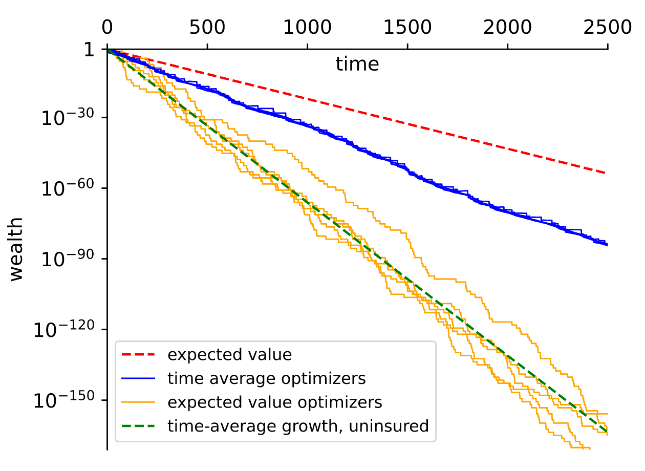
Peters (2023) argues that we can think of insurance as a tool to make wealth grow faster rather than as protection for the risk averse. This plot shows the outcomes for agents facing a 5% probability of a loss of 95% of their wealth each period. Uninsured agents experience ruinous path over time, losing far more than would be implied by the expected value. Those who insure at a cost experience a slower decline.

As an aside, I do find these numbers quite comical: 2500 periods with a 5% probability of loss, leading to an expected value of around 10^{-70} times the initial wealth even under the insured scenario. The expected-value optimisers, even if they stated with every atom in the universe, would be left with a fraction of an atom by the end.

Peters and Adamou (2022) similarly propose a desire to maximise the growth rate as the origin of cooperative behaviour. Here, the green trajectories are the selfish agents, the blue line the cooperators. In some ways, this is just the insurance problem reframed.

One of the more interesting examples concerns time preference. Adamou et al. (2021) use growth rate maximisation as an explanation for exponential discounting, hyperbolic discounting and preference reversals, depending on the particular wealth dynamic.

I won’t cover all the scenarios, but this image captures a situation where an agent in an additive world has a choice between a smaller sooner and a larger later pay-off. This agent seeks to maximise the growth rate of their wealth. From the perspective of t_0 the larger later pay-off provides a higher growth rate, which is equal to the slope of the line extended to the top of that pay-off. By the third frame, as the agent moves closer to the smaller, sooner pay-off, the higher growth rate now comes from that early pay-off. They have reversed their preference.

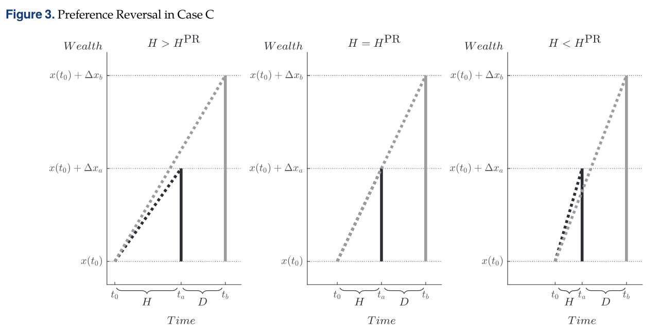
It is when seeing ideas such as this that the suggestion that ergodicity economics is a “psychology free” seem slightly ridiculous. The agent must be myopic to be unable to see their upcoming preference reversal, or to realise the foregone larger opportunity on the other side of that smaller sooner payment.

The experiment

But rather than going down that rabbit-hole, I want to present an experimental result. In 2019, a working paper was released examining whether shifting between an additive and multiplicative environment would change risk preferences. One of my blog posts was on that working paper. The paper was ultimately published in 2021 in PLOS Computational Biology (Meder et al., 2021).

That first experiment was subject to many criticisms, including by me, so Skjold et al. (2024) designed a new experiment. A pre-print describing the results from this experiment was released at the end of May. Some of the criticisms have been addressed in this new experiment, and the result is interesting.

Experimental participants were randomised to an additive or multiplicative environment where they were asked to make a series of bets. After making the bets in one environment, they were crossed over to the other.

At the beginning of the additive and multiplicative session, participants were trained on a set of fractal images, each of which had a specific effect on their endowment: multiplication by some fraction in the multiplicative session, or addition or subtraction of some sum in the additive session. Participants were then tested on whether they had learnt the ordering of the fractals, with the subset of participants with low learning excluded from the analysis. This image shows the training procedure, which essentially comprises exposure to the fractal and then an update to their wealth.

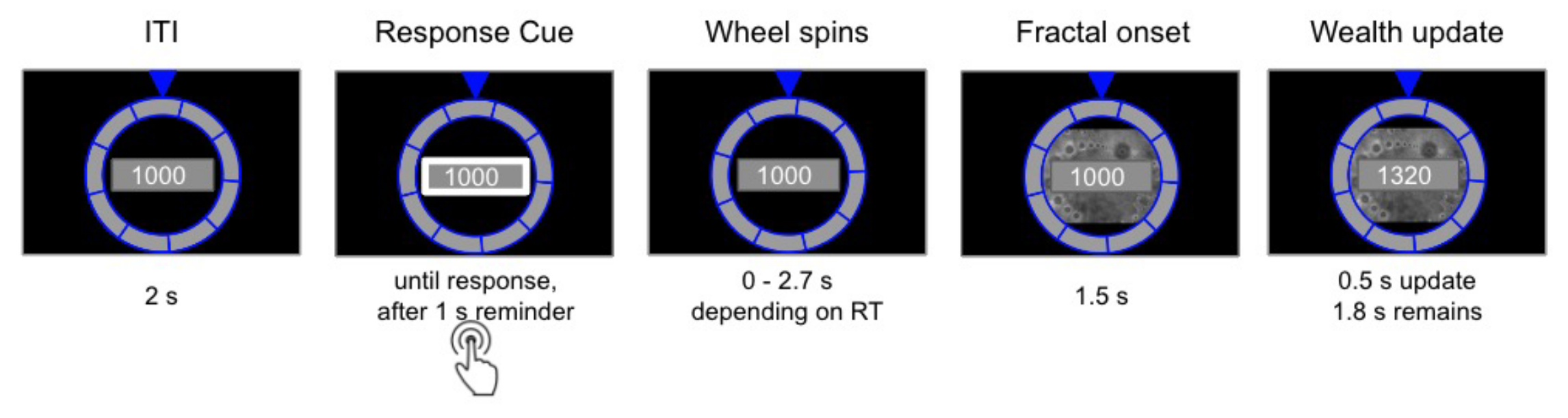
This use of fractals instead of numbers is one of the confounding factors that could influence the results: we have introduced ambiguity into the subsequent decisions. It was one of my critiques of the original experiment, but I clearly wasn’t very persuasive. Anyhow, let’s ignore that for now.

Participants then proceeded to their decision task, where they had to choose between gambles, each of which is represented by two of the fractal images. Over a sequence of 160 decisions, they would be shown the gambles, make their choice, be shown the outcome of the gamble, then see the effect of the outcome on their wealth.

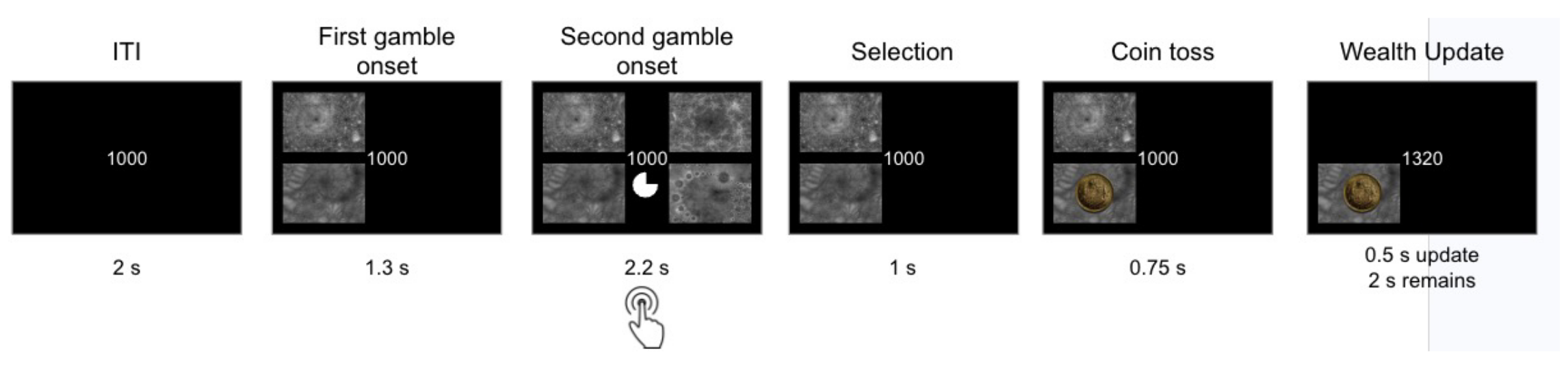
You can watch a video of the training and decision task below. (I didn’t show this video in the presentation.)

Participants were incentivised by being paid their relative proportion of points compared to a rolling window of 10 participants. Another exhibit of “why do we make experimental incentives so complicated” and another confound to the experimental result. By rewarding on proportional access to a pool, they have introduced diminishing gains and a cap on winnings. But again, I’ll ignore that for today.

So, to the result. The research team modelled participants as having an isoelastic utility function (a reasonably strong assumption), with the parameter \eta calculated by Bayesian cognitive modelling.

f_{\eta}(x)=\begin{cases} \frac{x^{1-\eta} - 1}{1-\eta} & \text{if } \eta \neq 1 \\[6pt] \ln(x) & \text{if } \eta = 1 \end{cases}

What would we predict the value of \eta to be in this experiment? Expected utility theory is quiet on the precise value. The ergodicity economics approach, however, gives us a prediction. First, \eta will be one in the multiplicative condition, as log utility maximises the growth rate. Second, \eta will be zero in the additive condition. The growth rate is maximised in an additive environment by risk neutral behaviour.

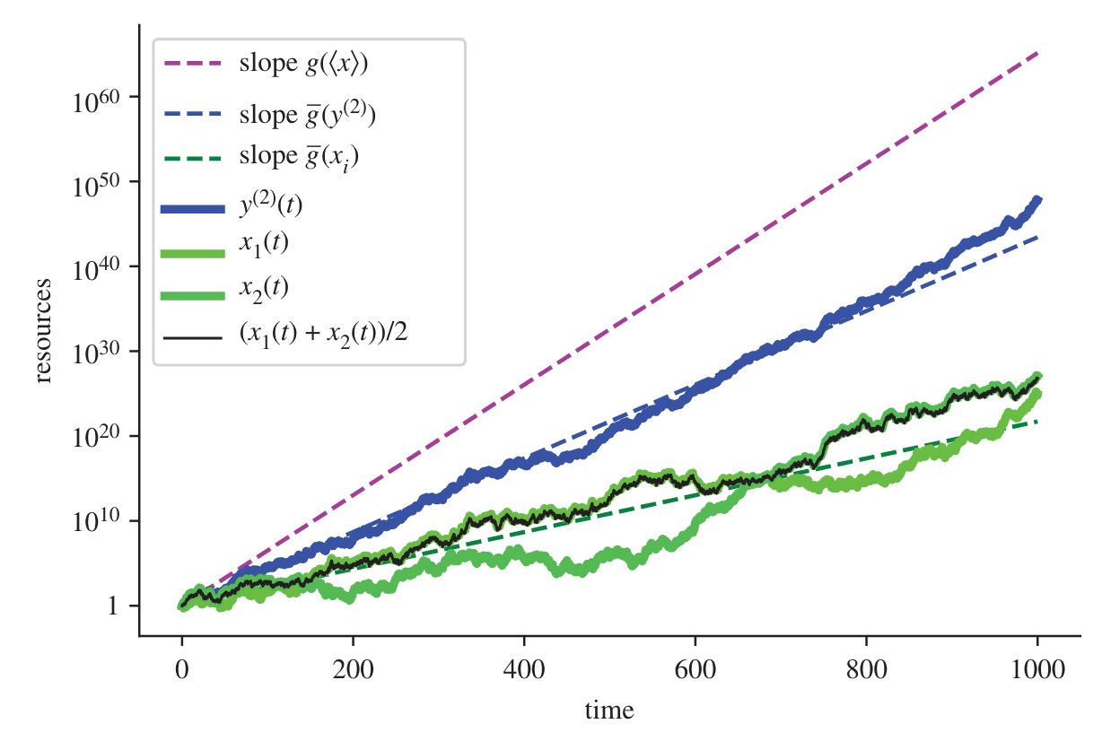
This chart shows the result. Thin lines represent individual participants. The thick lines represent the aggregate. For the additive scenario, participants were close to risk neutral: the aggregate estimate of \eta was 0.1. For the multiplicative condition, although there was a wider distribution of values, the central estimate of \eta was one.

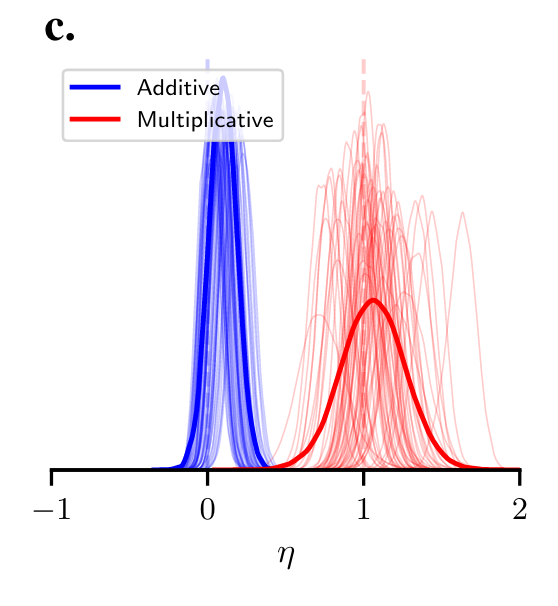
Despite the elements of this experiment that I would do differently - I have only hinted at a couple - this is a strong result.

If the ergodocity economics hypotheis is correct, it is worth thinking about what this means psychologically.

When modelling the utility function, the researchers took the value of x to be the participant’s experimental wealth at the time the participant makes their decision. It is the initial endowment, plus or minus the results of the previous bets. x does not include outside wealth.

But if this use of x is an accurate characterisation of the decision making process of the agents, it suggests a form of narrow bracketing or a degree of myopia. Agents are maximising the growth rate within the experiment, not more generally. We need to introduce some psychology to explain this. (This phenomenon is common across lab experiments involving risky decisions.)

Similarly, this experiment is part of a broader environment with either multiplicative or additive characteristics. Experimental participants can take their payment from the experiment and invest it. Maximising the growth rate in the additive condition by maximising expected value may not maximise the total growth rate if the world outside the experiment is multiplicative.

An evolutionary analysis

Now, via a rather long and winding path, I want to turn to a couple of evolutionary observations about ergodicity economics. There is a large literature in the evolution of preferences, not to mention in the evolutionary biology literature itself, that is relevant to an analysis of growth rate maximisation. Since the concepts are already there, I’m going to lean on them and turn them to my own purpose.

The first evolutionary angle concerns what happens when we take a gene’s eye view. And to assist me in making this point, let me show a quote from a Nature Physics paper in which Ole Peters (2019) summarises his work:

[I]n maximizing the expectation value - an ensemble average over all possible outcomes of the gamble - expected utility theory implicitly assumes that individuals can interact with copies of themselves, effectively in parallel universes (the other members of the ensemble). An expectation value of a non-ergodic observable physically corresponds to pooling and sharing among many entities. That may reflect what happens in a specially designed large collective, but it doesn’t reflect the situation of an individual decision-maker.

Ignoring the fact that Peters mis-characterises expected utility theory, this idea of interacting with copies of themselves is what happens at the level of genes. By the presence of multiple copies of a gene across individuals, the gene can experience the ensemble average. The following toy model and simulation illustrates.

A toy model

Suppose two types of agents lived in a non-ergodic world.

One type of agent seeks to maximise the time-average growth rate of its number of descendants. This desire to maximise the time-average growth rate is a function of its genotype, and is transmitted to its children.

The other type of agent seeks to maximise the expected number of offspring. Similarly, this agent’s preferences are set genetically.

In the environment in which these agents live, they have a choice of strategy. One strategy is to have a single offspring asexually with certainty before they die. The other strategy is a 50:50 bet of having either 0.6 or 1.5 offspring. Part offspring sounds weird, but with a large population of agents, you can think of this as the average number of offspring. The simulation works out largely the same if I make the number of children probabilistic in accord with those numbers. You can see I have effectively mimicked the classic ergodicity economics bet.

One final feature in this environment will be that each individual experiences its own flip. You might think of this environment as involving idiosyncratic risk. This is an important assumption that I will return to.

Given this setup, the type that maximises the expected number of offspring always accepts the bet. The time-average growth maximiser always rejects it. Which would come to dominate the population?

The time-average growth rate maximiser population stays constant. One offspring to each asexual parent.

This is a chart of the population of the accepting type for a simulation of 100 generations, starting with a population of 10,000.

set.seed(20240705)

# create function to round probabilistically - important when small numbers involved
probabilistic_round <- function(x) {
  if (runif(1) < x - floor(x)) {
    ceiling(x)
  } else {
    floor(x)
  }
}

# Function to simulate evolution betting
evolutionBet <- function(p, n, t, gain, loss) {
  
  #p is probability of a gain
  #region  is how many people in the simulation
  #t is the number of generations simulated
  
  params <- data.frame(value = c(p, n, t, gain, loss))
  rownames(params) <- c("p", "n", "t", "gain", "loss")

  sim <- numeric(t + 1)
  sim[1] <- n # Start population

  for (i in 1:t) {
    for (j in 1:round(n)) {
      outcome <- rbinom(1, 1, p)
      n <- n + (ifelse(outcome == 1, gain, loss) - 1)
    }
    n <- probabilistic_round(n)
    sim[i + 1] <- n
    if (n == 0) break
  }

  sim <- data.frame(period = 0:t, n = sim)
  list(params = params, sim = sim)
}

evolution <- evolutionBet(p=0.5, n=10000, t=100, gain=1.5, loss=0.6) #more than 100 periods can take a very long time, simulation slows markedly as population grows

# Plot the population growth for the evolutionary scenario (Figure 8).

basePlotEvo <- ggplot(evolution$sim[c(1:101),], aes(x=period))

expectationPlotEvo <- basePlotEvo +
  geom_line(aes(y=n), color = 1, linewidth=1) +
  labs(y = "Population")

expectationPlotEvo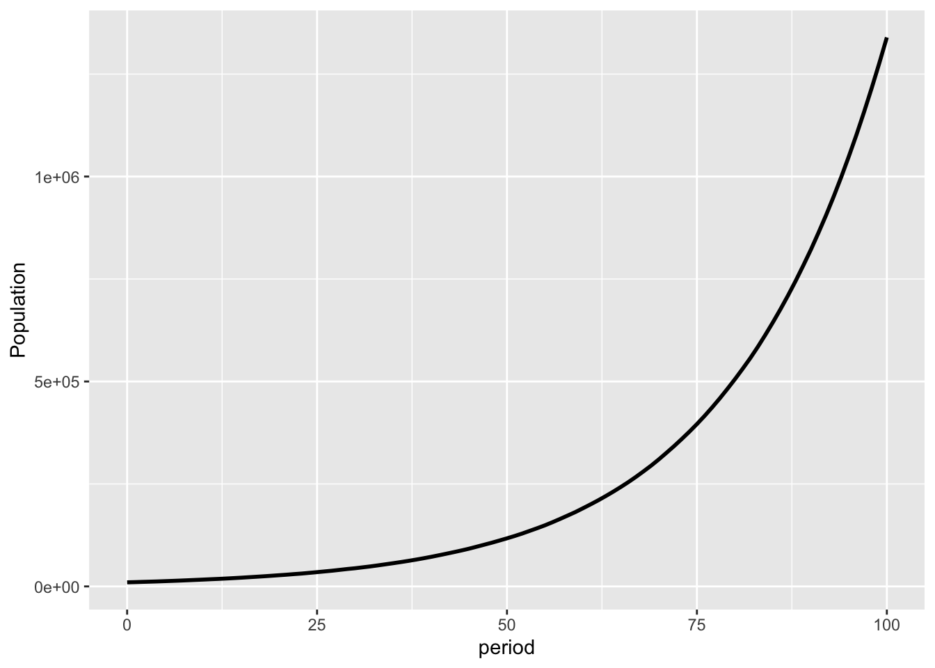

Figure 4: Population of accepting types

You can see that they have a population growth rate of close to 5%.

Why don’t they experience the decline we saw in earlier simulations of this bet? Because their copies experience the full ensemble of outcomes.

So here we have a toy model that shows that time-average growth rate maximisation may not be the optimal strategy in a multiplicative environment. The constant population of time-average growth rate maximisers is swamped by the spreading population of the expected value maximisers.

This behaviour could also emerge where it did not previously exist. The simulation I just showed you had 10,000 agents with expected value maximising behaviour to start. What if we had a population of time-average growth rate optimisers, and a single expected value maximiser emerged?

I simulated 10,000 instances of a single individual developing the mutation. This plot shows the population of the first ten mutants. For five of them, the mutation appears and disappears. For the other five, however, they grow into a substantial population.It only takes a few agents with this mutation to effectively diversify the results.

# run 9 simulations with 1 accepting type to start

set.seed(20240705)

mutations <- 10000

for (i in 1:mutations) {
  assign(paste0("evolution_", i), evolutionBet(p=0.5, n=1, t=100, gain=1.5, loss=0.6))
}

# Create a data frame for each simulation and store in a list
data_frames <- list()

for (i in 1:mutations) {
  # Dynamically retrieve the variable and select the first 101 rows of $sim
  current_data <- get(paste0("evolution_", i))$sim[1:101, ]
  
  # Add a column for 'i' to use as color in plotting
  current_data$i <- i
  
  # Append to the list
  data_frames[[i]] <- current_data
}

# Combine all data frames into one
combined_data <- do.call(rbind, data_frames)

# Count the number of simulations where the mutation spread (where n > 1 when i = 100)
mutation_count <- sum(combined_data[combined_data$period == 100,]$n > 1, na.rm = TRUE)

# Plot first 10 lines
mutationPlotEvo <- ggplot(combined_data[combined_data$i >= 1 & combined_data$i <= 10,], aes(x=period, y=n, color=factor(i))) +
  geom_line() +
  labs(y = "Population") +
  #remove legend
  theme(legend.position = "none")


mutationPlotEvo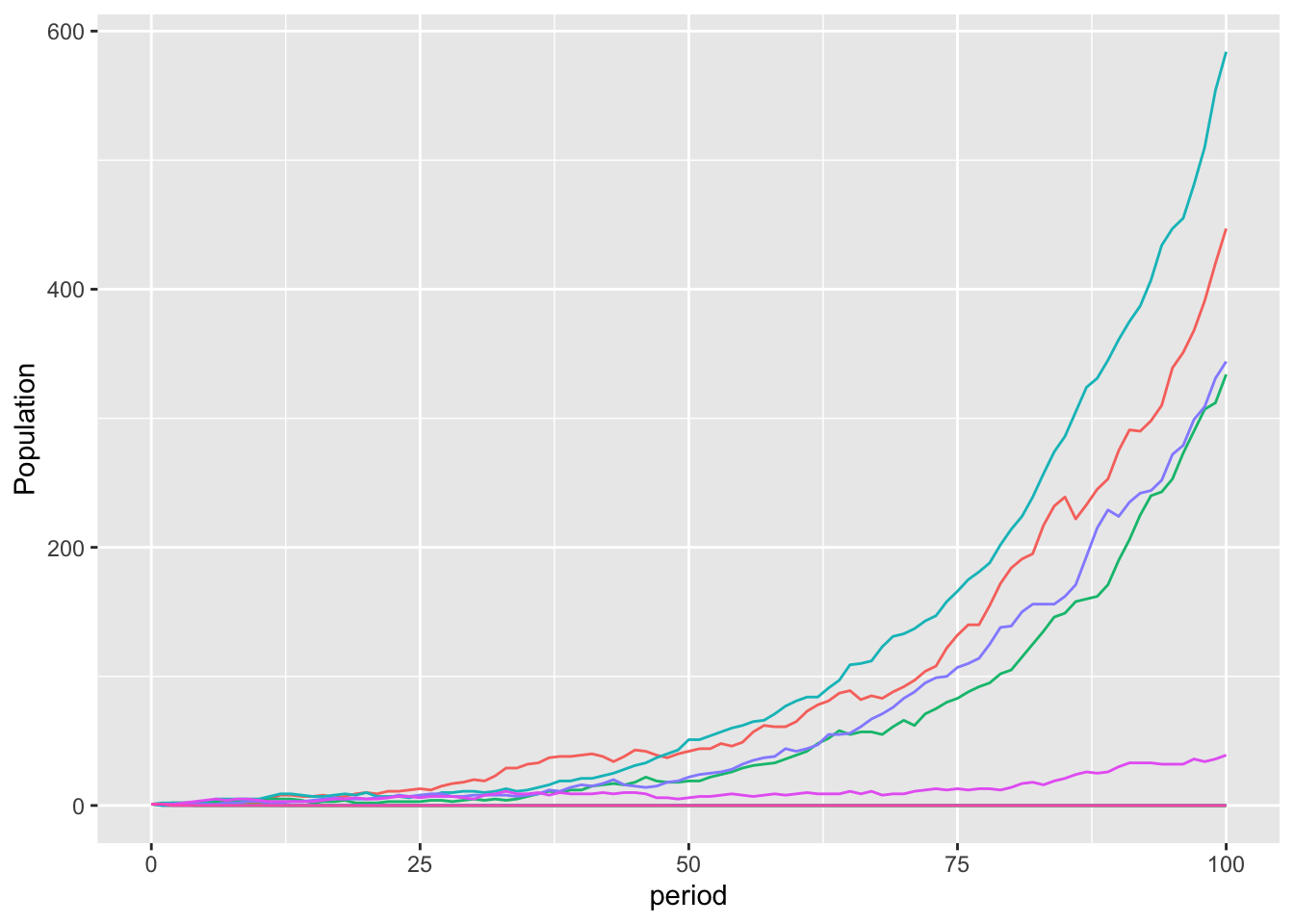

Figure 5: Population of accepting types with mutation

If we zoom into the first 35 periods, you can see the dynamic for those where the mutation did not spread.

# Plot first 35 periods only
mutationPlotEvo30 <- ggplot(combined_data[combined_data$i >= 1 & combined_data$i <= 10,], aes(x=period, y=n, color=factor(i))) +
  geom_line() +
  labs(y = "Population") +
  xlim(0, 30) +
  ylim(0, 35) +
  #remove legend
  theme(legend.position = "none")

mutationPlotEvo30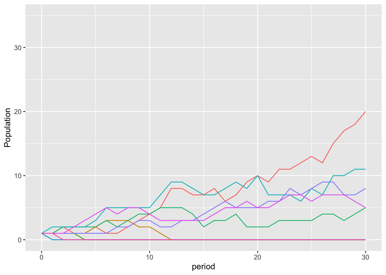

Figure 6: Population of accepting types with mutation (first 30 periods for first 10 agents)

This is a slightly rosier picture than occurs across the full 10,000 simulations, where the mutation did not spread 70% of the time.

These illustrations suggest that time-average growth optimisation may not be the optimal strategy, but it hinges on one critical assumption: that risk is idiosyncratic. Diversification enables the gene to experience the ensemble average. What if such diversification is not possible?

In that case, we are effectively back to the world that I showed you at the beginning. You could consider each line to represent an individual and their children, with their children all bound to the same bet. In almost all cases, this leads to a decline in frequency. An extraordinarily lucky few might boom through many rolls of the dice, but that is a rare chance.

Further, recall decline toward the end of the 100 periods. This occurred as a small number of genetic lines comprise most of the population - in fact, one single line of the original 10,000 comprises 53% of the population at the end of 100 periods - and they cannot diversify their risk. A few unlucky coin flips and they are gone.

The result is that, over a long enough time horizon, everyone is wiped out. There is no longer a lucky few. Here’s the same simulation plotted through 1000 iterations, over evolutionary time, in both linear and log scales.

nonErgodicPlot <- plotWealth(sim=nonErgodic, t=1000, people=20)
nonErgodicPlot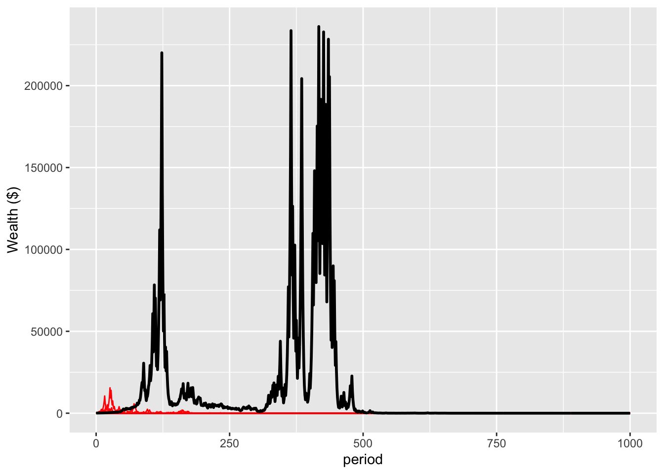

Figure 7: Population of accepting types over 1000 periods

logNonErgodicPlot <- nonErgodicPlot+
    scale_y_log10(breaks = c(0.0001, 0.1, 100, 100000), labels = c("0.0001", "0.1", "100", "100000"))
logNonErgodicPlot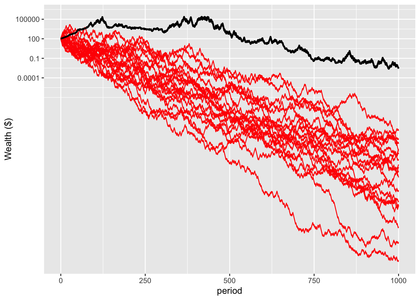

Figure 8: Population of accepting types over 1000 periods (log scale)

The result is that with aggregate risk, time-average growth rate maximisation can be the optimal strategy.

Probability matching

To explore this in more detail, I’m going to turn to another example that has a rich history in the biology literature.

The particular example I am going to pick is a bit cartoonish, and comes from Andrew Lo’s Adaptive Markets. This in turn draws on a more technical paper by Thomas Brennan and Lo (2011) published in The Quarterly Journal of Finance to explain the evolution of probability matching. You can find other earlier examples in the literature, such as by Cooper and Kaplan (1982) in The Journal of Theoretical Biology.

The example concerns an animal called the tribble. For amusement, I chucked an earlier draft of this presentation into ChatGPT and asked it to illustrate it. Most of what it produced was unusable, but I’ve kept a couple of images for which I thought it did a good job.

Tribbles live in a region comprising valleys and plateaus. Tribbles reproduce once in their life (producing three offspring asexually) and must choose whether to reproduce in the valley or on the plateau. This is a risky decision, however, as the valleys are affected by floods and the plateaus by drought.

Each generation there is a 75 per cent probability of sun. In such a case, the tribbles born on the plateau perish. The other 25 per cent of the time, it rains, leading to flood in the valleys and the death of those tribbles breeding there.

What, then, is the growth maximising breeding strategy?

Let’s set q as the proportion of tribbles that breed in the valley. If we maximise the expected number of offspring, tribbles would breed in the valley 100 per cent of the time. That is, q=1, leading to an an expected 0.75\times 3=2.25 offspring.

However, in the long run, if all tribbles make this choice, the tribbles will be wiped out. Over the long term, the tribbles will experience droughts 75 per cent of the time and floods 25 per cent of the time. Putting this into the language of ergodicity economics, the time average growth rate is zero.

To find the q that maximises the growth rate, we take the log of G and calculate the derivative. The solution is to breed in the valley 75 per cent of the time and on the plateau 25 per cent of the time.

\begin{align*} G&=3\times q^{0.75}(1-q)^{0.25}\\[6pt] \\ \log(G)&=\log(3)+0.75\log(q)+0.25\log(1-q)\\[6pt] \\ \frac{d}{dq}\log(G)&=\frac{0.75}{q}-\frac{0.25}{1-q}=0\\[6pt] \\ q&=0.75 \end{align*}

Probability matching in this world maximises the time-average growth rate.

This result is the same if we approach this from the perspective of log utility. If we maximise log utility as a function of number of offspring, we get the same value of q.

\begin{align*} U(n)&=0.75\times \log(3q)+0.25\times log(3-3q))\\[6pt] \\ \frac{d}{dq}U(n)&=0.75\times \frac{3}{3q}-0.25\times \frac{3}{3-3q}=0\\[6pt] \\ q&=0.75 \end{align*}

Here we have a world where maximising the time-average growth rate is the optimal solution. In this case, it is achieved via probability matching.

There is one feature of this scenario that might seem off. Probability matching maximises the growth rate for the species. But which individuals are heading off to the plateau where 75% of the time they are going to be fried? If this an altruistic act for the benefit of the species? Why not head down to the cool valley where they, as an individual, is more likely to survive?

The answer was provided by Grafen (1999). Suppose we have a large population of size N. If an agent heads to the valley, the expected fraction of the population comprising their offspring (\pi) will be:

\pi(\text{valley})\approx\frac{0.75}{qN}=\frac{1}{N}

If they stay to fry on the plateau, their offspring will comprise a similar fraction of the smaller remaining population:

\pi(\text{plateau})\approx\frac{0.25}{(1-q)N}=\frac{1}{N}

Fitness is a relative measure. At equilibrium q, each option delivers the same fitness.

Idiosyncratic versus aggregate risk

I have created two hypothetical worlds, one making the case for maximising expected value despite being in a multiplicative world, and another where maximising the time-average growth rate is the optimal strategy. In both cases, the optimal strategy relies on the gene’s eye view. The variation comes from the probability structure of the environment.

I am hardly the first to propose this. I’m drawing on a rich history of research into the evolution of geometric growth rate maximisation in the biological literature. This in turn has been used by economic researchers such as Robson and Samuelson (2011) in the analysis of the evolution of preferences.

But, I like to think that this ergodicity economics exercise provides a nice opportunity to tie multiple threads together to provide a different perspective.

What’s next? I’ve been building a set of simulations examining mixed environments. What if the probabilistic structure of the environment is a mix of multiplicative and additive bets? You could think of the additive phase of the experiment I described earlier as comprising an few additive gambles in a multiplicative world. What if the environment switches between additive and multiplicative?

There isn’t a simple closed form solution to this problem. If you have a mix of additive and multiplicative bets, or even a non-constant multiplicative growth rate, an “ergodic observable” cannot easily be created. At present, it is best examined via simulation.

References

Adamou, A., Berman, Y., Mavroyiannis, D., and Peters, O. (2021). Microfoundations of discounting. Decision Analysis, 18(4), 257–272. https://doi.org/10.1287/deca.2021.0436

Brennan, T. J., and Lo, A. W. (2011). The origin of behavior. The Quarterly Journal of Finance, 01(01), 55–108. https://doi.org/10.1142/S201013921100002X

Cooper, W. S., and Kaplan, R. H. (1982). Adaptive “coin-flipping”: A decision-theoretic examination of natural selection for random individual variation. Journal of Theoretical Biology, 94(1), 135–151. https://doi.org/10.1016/0022-5193(82)90336-8

Doctor, J. N., Wakker, P. P., and Wang, T. V. (2020). Economists’ views on the ergodicity problem. Nature Physics, 16(12), 1168–1168. https://doi.org/10.1038/s41567-020-01106-x

Ford, M. C., and Kay, J. A. (2023). The Limitations of Growth- Optimal Approaches to Decision Making Under Uncertainty. Econ Journal Watch, 20(2), 314–334. https://econjwatch.org/articles/the-limitations-of-growth-optimal-approaches-to-decision-making

Grafen, A. (1999). Formal Darwinism, the individualasmaximizingagent analogy and bethedging. Proceedings of the Royal Society of London. Series B: Biological Sciences, 266(1421), 799–803. https://doi.org/10.1098/rspb.1999.0708

Meder, D., Rabe, F., Morville, T., Madsen, K. H., Koudahl, M. T., Dolan, R. J., Siebner, H. R., and Hulme, O. J. (2021). Ergodicity-breaking reveals time optimal decision making in humans. PLoS Computational Biology, 17(9), e1009217. https://doi.org/10.1371/journal.pcbi.1009217

Peters, O. (2019). The ergodicity problem in economics. Nature Physics, 15(12), 1216–1221. https://doi.org/10.1038/s41567-019-0732-0

Peters, O. (2023). Insurance as an ergodicity problem. Annals of Actuarial Science, 17(2), 215–218. https://doi.org/10.1017/S1748499523000131

Peters, O., and Adamou, A. (2022). The ergodicity solution of the cooperation puzzle. Philosophical Transactions of the Royal Society A: Mathematical, Physical and Engineering Sciences, 380(2227), 20200425. https://doi.org/10.1098/rsta.2020.0425

Robson, A. J., and Samuelson, L. (2011). The evolutionary foundations of preferences* (J. Benhabib, A. Bisin, and M. O. Jackson, Eds.; Vol. 1, pp. 221–310). North-Holland. https://doi.org/10.1016/B978-0-444-53187-2.00007-3

Skjold, B., Steinkamp, S., Connaughton, C., Hulme, O. J., and Peters, O. (2024). Ergodicity transformations predict human decision-making under risk. https://doi.org/10.31219/osf.io/c96yd